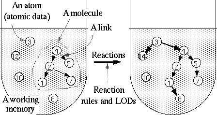
Figure 1. The elements of CCM
Paper number: 495
Last updated on April 1, 1995.
Note: The original version of this paper was presented at SuperComputing '95. A newer version of this paper may be found at http://www.rwcp.or.jp/people/yk/CCM/SC95/IndepPP.html (in HTML) or http://www.rwcp.or.jp/people/yk/CCM/SC95/IndepPP.ps (in PostScript).
The other problem of conventional methods is that they are very weak for unexpected situations because they are deterministic and explicitly designed, and thus, they cannot go beyond the human planner's explicit knowledge. Artificial systems in real world, such as on-line banking systems, are open to natural systems, i.e., human society or nature. Natural systems are autonomous and nondeterministic and thus their behavior is often unpredictable. Thus, artificial systems should be ready to process such unexpected situations, or at least they must be able to use implicit knowledge that the human planners do not know explicitly. However, deterministic and explicitly designed systems can, we believe, only process expected situations.
Thus, we should develop methods of problem solving which are not based on strict divide-and-conquer method and which are stochastic, or randomized, and thus, not deterministic. Not all methods that satisfy these conditions are suitable, of course. However, the methods that we should develop are, as we believe, among the methods that satisfies these two conditions, and not among the methods that are deterministic or based on strict divide-and-conquer method.
Kanada [Kan 92][Kan 94] proposed a computational model called CCM (Chemical Casting Model) [Kan W3], which is a model of stochastic and local- or partial-information-based computation. Local-information-based computation seems to have a chance to process unexpected situations using implicit knowledge that is emerged from interaction between local computation processes. Solving combinatorial problems, such as the N queens problem [Kan 94], graph or map coloring problem [Kan 93b][Kan 95b], traveling salesperson problems [Kan 93a], or fuzzy coloring problem [Kan 95a] has been experienced. However, it has been tested on sequential computers.
A method of parallel processing of solving combinatorial problems using CCM is proposed in the present paper. A problem is solved using multiple independent processes in this method. The word, ``independent,'' means that the processes do not communicate each other. This method is stochastic or randomized. This method is not based on divide-and-conquer method in the conventional sense. No search tree is built in this method. This method can be regarded as a problem-solving method based on implicit and stochastic divide-and-conquer. It is not yet certain that this method lead to a problem solving method that is holistic and adaptive to natural systems. However, we think that there is possibility.
The computational model, CCM, is briefly explained in Section 2. A method of combinatorial problem solving using CCM is explained in Section 3. A probabilistic model of CCM-based computation, which is called the Markov chain model, is explained in Section 4. The method of independent parallel processing using CCM is explained in Section 5. The results of experiments on this method are shown and analyzed in Section 6. Related work is mentioned in Section 7. Finally, conclusions are given in Section 8.
CCM has been developed for emergent computation [For 91][Lan 89-94], which is computation based on local and partial information. CCM is based on a production system. Production systems are often used for developing expert systems or modeling human brains. However, CCM is different from conventional production systems. Firstly, evaluation functions, which are evaluated using local information only, are used. Secondly, stochastic control, or randomized ordering of rule applications, is used. Production rules are also applied only using local information.
The system components in CCM are shown in Figure 1. The set of data to which the rules apply is called the working memory. A unit of data in the working memory is called an atom. An atom has a type and an internal state, and may be connected to other atoms by links. Links are similar to chemical bonding, but the difference is that links may have directions. Any discrete data structures such as lists, trees, graphs or networks can be represented using atoms and links.
The state of the working memory is changed locally by reaction rules. ``Locally'' means that the number of atoms referred by a reaction rule is small [*1]. The reaction rules are written as forward-chaining production rules, such as rules in expert systems. However, reaction rules are at a lower level, or more primitive, than rules in expert systems. So, the reaction rules are more similar to reaction formulae in chemical reactions, and thus, this model is called the chemical casting model. The syntax of reaction rules is as follows:

For example, the following reaction rule, which is a rough sketch, simulates the generation of water from oxygen and hydrogen:
The reaction rule can be activated when there is a set of atoms that matches the LHS patterns. If the reaction rule is activated, the matched atoms vanish and new atoms that match the RHS patterns are generated. A single reaction rule is enough for solving a simpler optimization or constraint satisfaction problem like the graph vertex coloring problem, which is described later, or the 0-1 integer programming problem. Two or more reaction rules are needed in more complex systems, in which there are two or more ways of changing atoms.
Local order degrees (LODs) are a type of evaluation functions. An LOD is defined for an atom or a small number of atoms. Thus, it is different from a global evaluation function, such as that in simulated annealing or energy function of a neural network. A global evaluation function cannot be defined under open and nondeterministic environment in which the number of data is not fixed, but an LOD can be defined in such situation. LODs express the degrees of local ``organization'' or ``order.'' They are defined by the user to take a larger value when the local state of the working memory is better. An LOD may be regarded as a negated energy. For example, it is analogous to bonding energy in chemical reaction systems.
A reaction takes place when the following two conditions are satisfied. First, there exists an atom that matches each pattern in the LHS. Second, the sum of the LODs of all the atoms concerned in the reaction, i.e., the atoms that appear on either side of the reaction rule, does not decrease as a result of the reaction. Reactions repeatedly occur while the above two conditions are satisfied by a combination of any rule and atoms. The system stops, i.e., becomes a stationary state, when such a combination is exhausted. However, reactions may occur again if the working memory is modified because of changes in the problem or the environment. Thus, open and dynamic problems as mentioned beforehand can probably be handled properly using CCM.
Typically, there are two or more combinations that satisfy the two conditions at the same time. There are two possible causes that generates multiple combinations. One cause is that there are two or more collections of atoms that satisfy the LHS of a reaction rule. The other cause is that there are two or more reaction rules containing atoms that match the patterns in the LHS. In each case, the order of the reactions, or the order of selection of such combinations, and whether they occur in parallel or sequentially is determined stochastically or randomly. Therefore, although the microscopic behavior of CCM, i.e., a reaction, may be deterministic in a sense, the macroscopic behavior is nondeterministic or random.
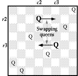
The N queens problem is an extension of the eight queens problem. The LOD and the rule in a visual form for the N queens system are shown in Figure 2. This system contains only one rule and a definition of the mutual order degree, o(x, y), i.e., an LOD defined between two queens. This rule swaps the rows of two queens (Queen2 and Queen3 in Figure 2). See Figure 3. Queen1, which can be called a catalyst, remains unchanged by the swapping. The role of the catalyst is explained later. No link is used in this rule. The value of LOD o(x, y) is defined to be higher (i.e., 1) when queens x and y are not diagonally oriented, and lower (i.e., 0) when they are diagonally oriented.
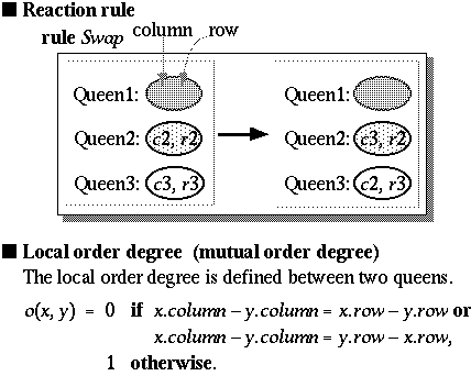
However, the rule shown in Figure 2 contains three patterns for queens both in LHS and RHS. The third pattern (i.e., Queen1 in Figure 2) does not change the contents of the working memory, but it affects the computation of order degrees. A reaction takes place when the following condition holds:
If the rule is executed with an appropriate initial state, the system repeats the selection of three queens and reaction of the instance. The initial state must satisfy the following condition: there is only one queen in each row and each column. The simplest layout that satisfies this condition is to put all queens on a diagonal line. If this condition holds, it holds at any time in the system because the reaction preserves the condition. The system stops when a solution of the N queens problem is found.
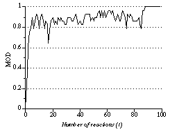
A mean value of LOD is called a mean order degree (MOD). An MOD can be local or global, i.e., a mean of either small or large number of data can be defined. An MOD can be defined in open environment in which the number of data is not fixed, on the contrary to the total of LOD or global evaluation functions. An MOD changes continually while solving a problem. A sample path of MOD time sequence is shown in Figure 4. The MOD shown in this figure is the mean value of the LODs of the eight (i.e., all the) queens. The value of MOD changes stochastically, but it increases in average and becomes the maximum value, i.e., 1, when the number of reactions is 88 in this case. This means that the system found a solution. The system becomes stationary when it finds a solution.
Other constraint satisfaction problems can be solved in the similar method as the N queens problem, if all the constraints are expressed as a relation between two objects [Kan 93b]. The values of LODs can be defined to be 0 or 1. Thus, the values of MODs are between 0 and 1. The values of MODs become 1 when the problem has been solved.
Time sequences of MODs can be approximated by a Markov chain in the processes of solving several problems, including the N queens problem and graph/map coloring problems, experimentally [Kan 93b]. MODs are asserted to take discrete values, o[0], o[1], ..., o[I] (0 = o[0] < o[1] < ... < o[I] = 1), here [*2]. Time is measured by the number of reactions from the beginning. The value of MOD at time t, O(t), is a random variable. The probability that O(t) is equal to o[I] is described as p(O(t) = o[i]), where the following condition holds:
 p(O(t) =
o[I]) = 1
In the case of the eight queens problem, the eigen values are estimated to be as follows [Kan 93b] by measurements [*3]:
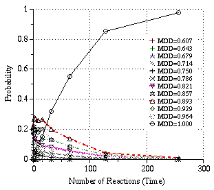
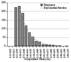
The probability of each MOD value is measured statistically in the case of the eight queens problem. The result is displayed in Figure 5. The probabilities of the states except the solution state, i.e., the state in which MOD = 1, decreased almost exponentially as expected. The distribution of computation time is measured statistically. The result is displayed in Figure 6. The distribution is close to an exponential distribution except when time (the number of reactions) is near zero [*3A]:
The method of parallel processing is as follows. (See Figure 7.) A parallel computer with at least M processors is used. Only one process runs on each processor. Thus, the processor and the process are identified in the present section. The same reaction rule and LOD are stored in each processor. The initial data may be the same or different for all the processors. The computation of each processor, which is based on CCM, is performed independently. Each processor generates independent random numbers for selecting data to be reacted. This independence is very important [*4]. When a process finishes the computation, the solution found by the process is outputted, and all other the processes are killed. Communication between processors is used only for this process termination, and is never used during the computation. If the distribution of sequential computation time is exponential, the performance will be improved in proportion to M by this method.
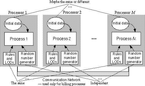
The reason why the acceleration is linear can be intuitively explained as follows. The computation can be regarded as a search of solution in combinatorial problem solving. Processes probably search different places in the search space, if the search space is large enough. So the efficiency is in proportion to the number of processors. The reason of linear acceleration is explained theoretically using the following theorem, in which the value of each random variable is interpreted as execution time.
Theorem: If random variables, X1, X2, ..., Xm, follows an exponential distribution, whose density function is p1(x) = l exp(-lx), then the random variable, min(X1, X2, ..., Xm), follows the exponential distribution, whose density function, pm(x), is equal to ml exp(-mlx).
Proof: The probability that the value of the random variable min(X1, X2, ..., Xm) is larger than x is expressed as follows.
 pm(y)
dy
 p(y)
dy)^m
 pm(y)
dy = (d/dx)exp(-mlx),
which means
pm(y)
dy = (d/dx)exp(-mlx),
which meansThe distribution of the parallel processing time using M processors is equal to pM(x) by this theorem. The expectation of random variable X' that follows distribution pM(x') is 1/M of the expectation of X that follows distribution p1(x). Thus, the average parallel processing time is 1/M of the sequential processing time.
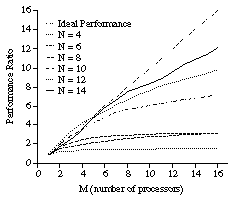
Parallel processing time of the N queens problem by the rule and LOD shown in Figure 2 has been estimated using 50 measurement results of sequential processing time. Namely, sequential processing time is repeatedly measured using computational language called SOOC [*5] and its interpreter, and the average of minimum values of 2 to 16 measured values are computed. The initialization time, i.e., the time for making initial placement of queens, is excluded from the measured time. The i-th measured execution time of the N queens problem is denoted by t(N, i) here (i = 1, 2, ..., 50). The average values of t(N, M, j) ( j = 1, 2, ...), which represents a measured value for the N queens by M processors, are plotted for M = 1, 2, 4, ..., 16, and N = 4, 6, ..., 14, in Figure 8, where t(N, 2, 1) = min(t(N, 1), t(N, 2)), t(N, 2, 2) = min(t(N, 3), t(N, 4)), ..., and t(N, 4, 1) = min(t(N, 1), t(N, 2), t(N, 3), t(N, 4)), ..., and so on. Because the distribution of the execution time is close to an exponential distribution when N is larger, the performance is accelerated nearly linearly.
Real parallel processing time has also been measured using the same rule and LOD that are hand-coded using C on Cray Superserver 6400 (CS6400) [Cray W3]. CS6400 has shared memory, and thus, multiple threads (but not UNIX processes), which run on different processors but share memory, are used for this measurement. However, the shared memory is used only for initial data distribution, final data output, and process termination. There is a parent thread and it distributes the input data, i.e., the value of N, to M child threads. Only the thread that finds the solution first outputs the solution and synchronizes with the parent. (The parent is busy-waiting for this synchronization.) Then the parent terminates and other threads are killed by the operating system. Thus, the threads are not explicitly killed in the program. The measured time includes the initialization time because the initialization is also performed in parallel and it is difficult to be separated.
Each thread computes random numbers independently
(using rand_r library routine). The random number seed
is generated using both the time in micro second and the
address of input data for each thread. I have chosen the
method of seed generation carefully to guarantee the independence
of random numbers between threads.
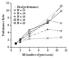
The execution time has been measured 50 times for each N. The result of measurement is shown in Figure 9. The CS6400 used for the measurement has 12 processors, each of which a thread is assigned to, and there is a parent thread. Thus, the maximum value of M is 11, where the parent is not counted. The performance is worse than the simulation. When N = 14, the acceleration is nearly linear in the simulation, but it is far below linear in the real parallel execution. However, the acceleration is almost linear when N is 18 or 20. Thus, the method shown in the previous section has been proved to be effective for the N queens problem. The reasons that the performance is worse than the simulation are probably as follows.
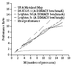
Computation of solving the graph or map coloring problem is also evaluated by the method using simulation [*7]. The simulated performance is shown in Figure 10. The performance of the USA mainland map [Tak 92] is not good probably because the problem is too small for parallelization. However, the performance of several problems in the DIMACS benchmarks [Tri W3][DIM W3] is good, and this method has been proved to be effective for the coloring problems.
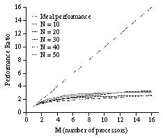
Not all constraint satisfaction problems are linearly accelerated by this method. Even the performance of the same problem can be different, if a different set of rules is used. For example, a simulated performance of the N queens problem has been measured and is shown in Figure 11. In this measurement, a rule that is different from Figure 2 and that has less locality is used. This rule refers a vertex and all its neighbors. This rule refers more data than the rule shown in Figure 2, i.e., it is less local. The ratio of performance improvement is less than 3 even when M = 16 and N = 50. This result shows that the high degree of locality in the computation is indispensable for performance improvement. The real parallel performance has not been measured because much improvement is not expected.
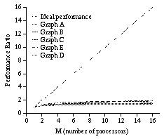
Other problems, including exchange sort and traveling salesperson problem (TSP), are also tested by simulation. The execution time of exchange sort, which can be regarded as a constraint satisfaction problem, is almost constant. Thus, it is almost never accelerated. The simulation results of TSP with 10 to 20 cities are shown in Figure 12. The acceleration ratio is far less than 2, even when the number of processors is 16. No global optimization problem that can be accelerated nearly linearly has yet be found. It is probably difficult to improve the performance of solving global optimization problems by this method because of non-local nature of their computation; they are global optimizations.
Several non-conventional stochastic problem solving methods for solving constraint satisfaction problems or satisfiability problems using a global evaluation function have been developed by Minton [Min 92], Selman [Sel 92], Gu [Gu 93] and others. These method have similarities to CCM-based method. The method of parallel processing shown in this paper may also be applied to them.
The result shown in the present paper is only one step toward the goal. Linear acceleration is possible only when the sub-problems are independent. However, we believe that researches on such implicit stochastic divide-and-concur methods will lead us to a new methodology of problem solving and software development, which is not only applied to parallel processing, in future.
[DIM W3] Center for Discrete Mathematics and Theoretical Computer Science, http://dimacs.rutgers.edu/.
[For 91] Forrest, S., ed.: Emergent Computation, MIT Press, 1991.
[Gu 93] Gu, J.: Local Search for Satisfiability (SAT) Problem, IEEE Trans. on Systems, Man, and Cybernetics, 23:4, 1108-1129, 1993.
[Kan 92] Kanada, Y.: Toward a Model of Computerbased Self-organizing Systems, Proc. 33rd Programming Symposium, 1992 (in Japanese. HTML and PostScript versions in Japanese at http://www.rwcp.or.jp/people/yk/Papers/CCM-papers-j.html#ProgSymp92 are also available).
[Kan 93a] Kanada, Y.: Optimization using Production Rules and Local Evaluation Functions, 11th Meeting of the Technical Group on Software Engineering, The Society of Instrument and Control Engineers (SICE), 1993 (in Japanese. HTML and PostScript versions in Japanese at http://www.rwcp.or.jp/people/yk/Papers/CCM-papers-j.html#SICE9302 are also available).
[Kan 93b] Kanada, Y.: Computations as Stochastic Processes -- Necessity and Examples of Macroscopic Models of Computation Processes --, IEICE Technical Groups on Computation / Software Science, COMP92-93, SS92-40, 1-10, 1993 (in Japanese. HTML and PostScript versions in Japanese at http://www.rwcp.or.jp/people/yk/Papers/CCM-papers-j.html#SIGPRG9303 and English abstract at http://www.rwcp.or.jp/people/yk/Papers/CCM-papers.html#SIGPRG9303 are also available).
[Kan 94] Kanada, Y., and Hirokawa, M.: Stochastic Problem Solving by Local Computation based on Selforganization Paradigm, 27th Hawaii International Conference on System Sciences, 82-91, 1994 (HTML and PostScript versions at http://www.rwcp.or.jp/people/yk/Papers/CCM-papers.html#HICSS27 are also available).
[Kan 95a] Kanada, Y.: Fuzzy Constraint Satisfaction Using CCM -- A Local Information Based Computation Model, FUZZ-IEEE/IFES '95, (PostScript version at http://www.rwcp.or.jp/people/yk/Papers/CCM-papers.html#Fuzzy-CSP is also available).
[Kan 95b] Kanada, Y.: Large-Scale Constraint Satisfaction by Optimization of Local Evaluation Function with Annealing, to be published.
[Kan W3] Kanada, Y.: CCM (Chemical Casting Model) Home Page, http://www.rwcp.or.jp/people/yk/CCM/.
[Kar 69] Karlin, S.: A First Course in Stochastic Processes, Academic Press, 1969.
[Koe 78] Koestler, A. : JANUS, Hutchinson and Co. Ltd., 1978.
[Lan 89-94] Langton, C. G.: Artificial Life I, II and III, Addison Wesley, 1989, 1991 and 1994.
[Meh 85] Mehrotra, R., and Gehringer, E. F.: Superlinear Speedup Through Randomized Algorithms, 14th Int'l. Conf. on Parallel Processing, 291-300, 1985.
[Min 92] Minton, S., Johnston, M. D., Philips, A. B., and Laird, P.: Minimizing Conflicts: a Heuristic Repair Method for Constraint Satisfaction and Scheduling Problems, Artificial Intelligence, 58, 1992, 161-205, 1992.
[Sel 92] Selman, B., Levesque, H. J., and Mitchell, D. G.: A New Method of Solving Hard Satisfiability Problems, AAAI '92, 440-446, 1992.
[Tak 92] Takefuji, Y.: Neural Network Parallel Processing, Kluwer Academic Publishers, 1992.
[Tri W3] Tricks, M.: The Second DIMACS Challenge, http://mat.gsia.cmu.edu/challenge.html.
Updated references may be found at http://www.rwcp.or.jp/people/yk/CCM/SC95/IndepPP.html#references.
[*1] Because (physical) distance is not a factor in CCM unlike systems such as a chemical reaction system, ``locally'' does not mean the distance is small.
[*2] Kanada [Kan 93a] shows a method of constructing a Markov chain model when the MOD takes continuous values.
[*3] It is currently not possible to estimate the eigen values only from theories.
[*3A] Because the distribution is exponential, the computation time is not bounded. The worst case computation time is not our concern.
[*4] If the random numbers are not independent, the performance degrades. For exapmle, if all the processors use the same duplicated sequence of random numbers, they compute the same result. Thus, the performance is the same as using one processor.
[*5] SOOC is a computational language designed for experiments of CCM-based computation. SOOC is built on Common Lisp.
[*6] Time for killing threads is not included in the measured time, but it is known to be almost negligible when N is large. This overhead is measured to be 1% (when N = 18) to 3% (when N = 12) in average.
[*7] A rule with variable number of catalysts [Kan 94][Kan 95a] is used for this measurement.
[*8] The function of these two versions of programs are different. Thus, it is not fare to state that a super-linear acceleration was performed.