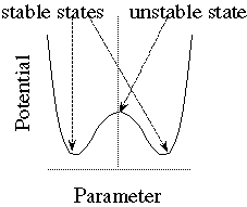
Prigogine [Pri 77] and Haken [Hak 78] pointed out that both determinacy and nondeterminacy are necessary for generating behavior of complex continuous physical systems, such as Bénard convection or Belusov-Zhabotinsky reaction system. I intend to show that this statement is also true in artificial life or complex discrete computing systems. Emergent computation without randomness in the computation process, such as that in synchronous CA, sometimes causes phantoms, which are phenomena that are so fragile that they almost never occur in real world where noise or randomness exists. Such a case may easily occur in a continuous dynamical system, as illustrated in Figure 1. If the potential of a system takes the minimal value, the system is stable. If the potential takes a value between the minimal and maximal value, the state of the system changes. However, if the potential takes the maximal value and no noise exists (or the temperature is zero), the system continues to stay in the unstable state. This does not happen in real world. Emergent computation without randomness may also fail to show their important features, which almost always occur in real world, in their behavior.
The type of CA, which is most widely used, is synchronous deterministic CA (e.g., [Wol 84]) as mentioned above. In this type of automata, randomness exists only in the initial state. However, there are two types of CA, in which randomness is introduced to their computation processes. The first type is CA with probabilistic (or randomized) state transitions (e.g., [Vic 89, Kau 84]). In this type of automata, the major source of randomness except the initial state lies in each cell. Thus, they can be called CA with local (or internal) noise. This type of automata has also been widely studied, because they are useful for simulating natural phenomena.[*1.1] The second type is random asynchronous CA [Ing 84, Lub 87, Hof 87]. In this type of automata, the major source of randomness lies in the order of state transitions of the cells, and thus, the noise is non-local or environmental to each cell.[*1.2] Ingerson and Buvel [Ing 84] compared patterns of synchronous automata and those of two types of random asynchronous automata, and found several interesting features of the latters. However, their observation and discussion is limited, and they do not distinguish the effects of randomness from those of asynchronism. Effects of non-local or environmental noise have not been deeply studied.
The objective of the present paper is to study random asynchronous CA more. The effects come from asynchronity and those come from randomness must be separated, and phantoms that are caused by noiselessness must be distinguished from real phenomena. A definition of one-dimensional asynchronous cellular automata (1D-ACA) is given in Section 2. Example patterns generated by 1D-ACA, in which the order of computation is randomized, and those generated by deterministic ones are compared in Section 3. The look-up table of 1D-ACA is interpreted and their properties, which are fully expressed only when stronger noise exists, is argued in Section 4. Very noise-sensitive (thus, phantom) patterns generated by 1D-ACA are discussed in Section 5. Conclusions are given in Section 6.